The Intuition behind Embeddings
Welcome to the first post of my blog! Today, I want to bring you the intuition behind embeddings a bit closer. Afterwards, I hope you will understand why they are used so widely and what they can actually learn.
The Story so Far…
To understand this, let’s first have a brief look at general machine learning models. At its core, every machine learning model tries to perform a certain task on a certain data set. That task might be analyzing an MRI image, detecting bots on Twitter, or recommending products to your customers. Therefore, the model perceives the data in some way and tries to find patterns in the data that facilitate its predictions. This perception is exactly what we want to have a closer look at. Usually, a data set consists of a huge set of individual examples like MRI scans, tweets, or user transactions. Each of the examples is represented as a set of features, e.g. image pixels, words in a tweet, or which user consumed which product. The model observes these examples one at a time by inspecting exactly these features. But where do we get the features from?
Traditionally, they are handcrafted by a human according to a fixed scheme. Let’s take the Twitter example as case of a Natural Language Processing (NLP) application. We first start with a vast set of tweets and look at each of them. We collect every unique word and put it in a huge dictionary which can easily contain tens of thousands of words in the end. Each tweet is then encoded as a so-called bag-of-word where each word is in its one-hot encoding: a word is represented as a giant vector of zeros (which has the same length as our dictionary) where exactly one value is 1, namely at the position of the particular word in the dictionary. Such representations are often called sparse. While it is easy to construct such one-hot encodings they have crucial disadvantages. The biggest problem is that words are essentially interpreted as an ID without any meaning attached. Let’s look at an example: when we look at the one-hot encoding of the two words cat and cats they get assigned a different ID. Hence, they are treated as completely different entities although their syntactic relationship is imminent.
What are Embeddings Actually?
Guess what could help to overcome these issues. You’re right, embeddings. The key idea is that we do not fix the representation of our examples by designing features. Instead we let the model decide which features are most helpful to fulfil the task. It chooses the features on its own - these learned features are called embeddings.
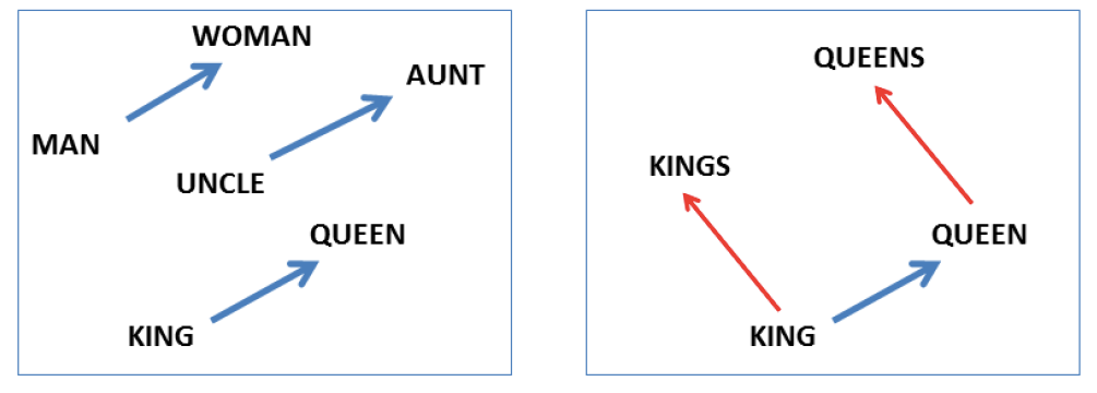
Let’s take a look at the probably most famous embedding model word2vec. In word2vec we try to find an alternative for our sparse one-hot encodings that contain more meaning. I don’t want to go into details how exactly these embeddings are obtained, but you can read this excellent blog post. The results are astonishing as the embeddings are syntacticly and semantically meaningful. This can be seen when playing a small analogy game, asking questions like “x is to y as z is to?”. A well-known example is “man is to king as woman is to” where word2vec would answer queen. This case is also visualized in the image below1. Besides semantic information, also syntactic information is captured, e.g. the information if a word is singular or plural. This would also resolve our issue with cat and cats.

Where Does the Word “Embedding” Come from?
Embeddings are essential vectors of real numbers. Each entry in this vector corresponds to a learned feature. The crux is that the length of the embedding vector is much smaller than a one-hot encoded vector (which has the same size as the dictionary). The name describes the act of embedding such a high-dimensional (e.g. one-hot encoded) entity into the low-dimensional space of the embeddings2. Sounds technical? Let me try to find a proper analogy: if someone asks you what defines you as a person, you could probably tell them quite a story. But if you are asked to describe yourself using only three words, you really have to think about what sets you apart, what “features” make you special. It is the same with embedding models: we ask the model to explain a complex issue (high-dimensional) but force it to use a compressed, simple (low-dimensional) answer. That way it really needs to focus on the most important parts and find features that properly explain the observed data.
Investigating the Embeddings
Word embeddings learned by word2vec or similar approaches are now ubiquitous in NLP and inspired dozens of other models. I want to give another fun example which produces surprising results. Last year, I participated in a Kaggle competition that aimed to understand the behaviour of customers of a music streaming platform. In particular, you had information about which user liked which song. The task was to predict exactly that for new combinations of users and songs - essentially building a recommendation system. You were given information about the user (like age, gender, on what platform the song was listened to etc.) as well as about the song (name, artist, length, genre, release date etc.). For the purpose of this blog, I trained an embedding model3 using only a subset of the features. The goal was not to build the perfect classifier but to illustrate the capabilities of embedding models.
The final model is trained using only the most crucial information, namely the user ID and the song ID - no additional meta data at all. Similar to the representation of words in NLP, we could as well use a one-hot encoding of our data. We would have two dictionaries of unique user and song IDs, respectively. Instead we are using an embedding approach: the model tries to find meaningful representations - embeddings - for both users and songs. To predict the preference of a user for a song, the model combines these representations in a specific way and produces a prediction. Again - we do not fix the representation of the input, instead we let the model decide what helps it the most.
After training, I have inspected the embeddings to find out if the model actually learned something meaningful about the music industry. Therefore, I have anaylzed the songs of different artists. More specifically, I have calculated an embedding for each of the 300 most popular artists (in my dataset) by simply averaging the embeddings of all his or her songs4. Let’s explore the embeddings by finding the five most similar artists5 to some popular interprets.
| Beyoncé | Jay-Z | Coldplay | David Guetta |
|---|---|---|---|
| Still Fresh (\(0.449\)) | Wiz Khalifa (\(0.434\)) | The Lumineers (\(0.676\)) | Pitbull (\(0.522\)) |
| France Gall (\(0.442\)) | Doc Gynéco (\(0.423\)) | Sofiane (\(0.479\)) | Showtek (\(0.447\)) |
| Mariah Carey (\(0.434\)) | Sam Smith (\(0.423\)) | U2 (\(0.447\)) | Mobb Deep (\(0.413\)) |
| Rihanna (\(0.418\)) | J. Balvin (\(0.407\)) | L.E.J (\(0.446\)) | Shakira (\(0.402\)) |
| Petit Biscuit (\(0.415\)) | Lil Wayne (\(0.392\)) | LP (\(0.436\)) | DJ Snake (\(0.373\)) |
The results really surprised me as the top 5 have a lot of reasonable choices6, I have emphasized the most relevant ones. Beyoncé is similar to Mariah Carey and Rihanna, all three famous women in Pop or R&B. Her husband Jay-Z produces hip hop music, consequently the US rappers Wiz Khalifa and Lil Wayne, as well as the French rap representative Doc Gynéco are present in his top 5. Also notable is the group of French house DJ David Guetta: Pitbull might not be directly in the same genre, but they have already featured in the same songs. Also further DJs, namely Showtek and DJ Snake, are placed near David Guetta.
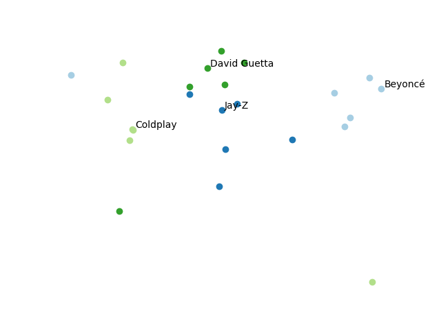
The following graphic visualizes the embedding of the four artists and their nearest neighbors which are colored accordingly. For this visualization, I used a dimensionality reduction technique called t-SNE. Again, you can see that similar artists cluster nicely together (with a few exceptions).

Of course, the rankings are not perfect as I still try to figure out how Sam Smith will fit in his hip hop neighborhood, but nevertheless the results are impressive. Please note again, there was absolutely no information about genres, features, or similar present during training - just user and song IDs. To explain the observed likes and dislikes, the model figured out some sense of genres, musical styles, and other information that is helpful for prediction. It was clearly able to induce some semantic meaning into the embeddings.
One weakness of embedding models is their interpretability: although you can compare e.g. the embeddings of different artists and verify their reasonability, it is really hard to interpret the embeddings themselves. The models do not provide human-interpretable captions for the learned features.
Conclusion
I hope you now understand the intuition behind embeddings: they are automatically learned features that capture the meaning of entities. Thus, they help a model to make better predictions and are used in a wide range of machine learning application, most prominently in NLP.
Image taken from Mikolov, T., Chen K., Corrado G., & Dean J. 2013a. Efficient Estimation of Word Representations in Vector Space. In ICLR WorkshopPapers. ↩︎
Embeddings are sometimes also called latent feature vectors as they are composed of “latent” features, i.e. features that are hidden in the data and cannot directly be observed. ↩︎
I have used a factorization machine which I will explain in more detail in an upcoming post. ↩︎
As an embedding is essentially a vector of real numbers which e.g. looks like this \([-0.526, 0.149, 0.123, ..., 0.141, -0.258, 0.161]\), it is easy to combine multiple embeddings by simply taking the elementwise mean. ↩︎
As measured by cosine similarity. ↩︎
Please note that the dataset seems to be from France, that’s why there is a small bias towards French artists. ↩︎